Factoring binomials using the greatest common factor

One way to factor binomials is by searching for the greatest common factor.

Consider

(5x * 25)

In this case the greatest common factor is 5 and the phrase can be written as

5(x*5)

Multiplying a trinomial by a binomial

Multiplying a trinomial by a binomial is a lot like multiplying a binomial by a binomial. You multiply the first term by all the factors of the second term, then multiply the outer(last) term by all the factors of the second term, then simplify.

Consider the example:

(x+5) (5x² + 3x + 6)

First we multiply our first term (x) by every term in the trinomial (5x² + 3x + 6)

this gives us:

(5x³ + 3x² + 6x)

next we multiply our outer term (5) by every term in the trinomial (5x² + 3x + 6)

this gives us:
(25x² + 15x + 30)

so we have
(5x³ + 3x² + 6x) + (25x² + 15x + 30)

we can simplify by adding like terms to get:
(5x³ + 28x² + 21x + 30)

Multiplying a binomial by a binomial

The most common way to multiply binomials is what is called the FOIL method

First
Outer
Inner
Last

Let us look at an example

(x+4) (x+1)

These are both binomials, to multiply them we first multiply the first two terms to get x²

Then we still take the first x and multiply it by the outer number: 1, to get x.

So far we have
x² + x

Now we do the inner number: 4

4 times x is 4x

and finally the last number 4 times 1 is 4

So in total we have
x² + x + 4x + 4

which can be simplified by combining the like x terms to

x² + 5x + 4

Polynomials

Polynomials can be anything from a single number to a variable to a combination of numbers and variables

Monomials have one term.
Such as... 8x⁴ , 6 , or 2xy

Binomials have 2 terms which are not like.
Such as... 2wz - 4dt , 4x² - 3x , 4c - 2d

Trinomials have 3 terms which are not like.
Such as... 4bt - 5yu + 9o , 3x² - 2x + 9 , 5t + 7y - 8u

Dividing exponents

Yesterday we learned that when you multiply exponents you add the number in the exponent, today we see that when you divide exponent you subtract the number in the exponent.

Consider

x⁷ / ³

What is this equal to?

x*x*x*x*x*x*x / x*x*x = x*x*x*x or x⁴

x⁷ / ³ = x^7-3 = x⁴

what about

x³ / ⁷

= 1 / x^7-3 = 1 / x⁴

We take the reciprocal because the exponent is greater in the divisor, or denominator.

Exponent

Exponents tell you how many times a factor is multiplied.

x * x * x (x times x times x)

Can be written as x³ or x^3 , when we write the multiplication in this way, we call it an exponent.

To multiply exponents we add them, for example, consider we have

x² * x³

what is this equal to?

x⁵

why is this? Well if we write it out, it becomes obvious


x² * x³

=


(x*x) * (x*x*x) or x⁵

if we have

5x² * 2x³

Then the bottom numbers (or base numbers) are multiplied, while the exponents are added


5x² * 2x³
=
10x⁵

Using Substitution to Solve a System of Equations

Suppose we had a system of equations

2x + y = 4
and
3x + 2y = 5

How can we solve for x and y?

The good thing is that we have two equations for two variables.

One way is to solve on equation for y and substitute. Let us start with

2x + y = 4

subtract 2x from both sides

y = 4 - 2x we can use this informaiton to solve for x by substituting y into the other equation

3x + 2y = 5 becomes

3x + 2(4-2x) = 5

3x + 8 - 4x = 5

-x = -3
x=3

so x = 3

Now we can substitute x into our first equation to find y

2x + y = 4

6 + y = 4

y = -2

To check let us substitute our answers into the equations and see if we get the same answer:


2x + y = 4
and
3x + 2y = 5

x=3 y= -2

2(3) - 2 = 4
6-2 =4 Correct.

Next

3(3) + 2(-2) =5
9 - 4 = 5 Correct.

So our solutions to the system check OK and are correct.

Systems of Linear Equations

A system of linear equations is a composed of two or more equations with the same variables.

If you have two variables then you need two equations
three variables - three equations, and so on.

Let say you have a system of two equations, if you were to graph the two equations
we would say the system has a solution where the two lines intersect.
If the two lines run parallel then there are no solutions.
If the two lines coincide, then they are the same, and there is an infinite number of solutions.

Linear vs non-linear equations

A linear equation is any equation which graphs a straight line and is of the form

Ax + By = C where A and B are not equal to zero.

examples:
3x + 5y = 8
(4/3)x + 6y = 0
x = 19

These are all linear equations.

Non-linear equations will not be a straight line, and are generally less intuitive, examples are

x^3 + 4y = 8 (this is exponential)

(5/x) + 3y = 9 (contains a variable in the denominator)

2xy = 8 (is multiplicative)

Solving inequalities

Inequalities are often represented in terms of

less than <
greater than >
and not equal to

I.E.:

3 < 4
4 > 3
4 not equal to 3

Like equalities, they can be solved by manipulating both sides

7 x < 21

divide both sides by 7

x < 3

-----------------

Consider

2 < 4

What if we multiply both sides by -2?

-4 < -8 ...but this is false!

So we must remember with inequalities that when we multiply or divide by a negative number we flip the sign!

-4 > -8 ...now correct!

Graphing linear equations the slope and intercept

Linear equations generally take the form

y = mx + b

m is considered to be the slope of the line
b is the y intercept

The smaller m is, i.e. m = 0.5 or 0.3 the steeper the slope.

Using formals to find information

Formulas are useful to give us information we may not be able to know otherwise.

Example:
D = rt

where
D = distance
r = rate
t = time

The formula gives us the distance we have traveled accounting for rate and time.

Consider:
We travel 70mph for 7 hours, how far have we gone?

D = 70 * 7 = 490 miles!

Since we know how to simplify expressions and solve for variables we can use the formula to answer many questions.

Consider:
How fast would we have to go to travel 490 miles in 7 hours?

490 = r * 7

r = 490 / 7 = 70 mph

Equations of the null and the infinite

Sometimes an equation will resolve to eliminate all its variables, this creates two results

1.Consider

5x + 25 = 5(x-50)

5x + 25 = 5x - 50

we subtract 5x from both sides and get

25=-50 or 0=75

In this case we know the equation doesn't make sense, since 0 is NOT equal to 75. When this happens we say the equation resolves to the empty set and that there is no solution.

2. Consider

5x + 25 = 5(x+5)

5x + 25 = 5x+ 25

we subtract 5x from both sides again

25=25 or 1=1

This solution is called the identity because the left side is exactly equal to the right side. You can substitute any number for x and arrive at the same answer, thus there are an infinite number of solutions. We can say that this equation resolves to the set of all reals, often notated as R.

Equations

Equations are statements that express equalities, typically using an = sign.

Such as
5=5
2+3 = 5
1+1+1+1+1=5

and so on.

Equations are useful because they can allow us to solve for missing variables in any real event we want to model

2x + 1 = 5

2x = 4

x=2

Simplifying Expressions and Combining Like Terms

In Math, like English, there is a desire to reach for simplicity and elegance when making statements.

Be as clear and short as possible to be effective.

Math expressions should be simplified, and one way to do this is to combine like terms, for example, we can realized that

2x + 3x + 2x + 10x = 27x , and it would be much better to write the shorter 27x

However

2x + 3y + 2x + 10y = 4x + 13y and that is as simple as we can get, because not all terms are like. That is to say, y is different from x and cannot be combined.

In the case of parenthesis expressions can be greatly simplified
2(2x + 4y) + 5(10x + 20y)

=

4x + 8y + 50x + 100y

=

54x + 108y

much simpler.

The ability to simplify expressions should not be underestimated. Math is used to model and describe real world problems, and its ability to be simplified allows us to draw insights from the world that would otherwise be obscured in complication.

Which way does the sign go?

The book I am working with makes a big deal about knowing which way the sign goes in operations of addition and subtraction.

I would say just try to work it out logically in your mind

3+4 = 7
3 + -4 = -1

This can get confusing when you subtract a negative number
3 - -4 = 7

This is probably one case where memorization works since it is hard to intuitively see that subtracting a negative number is the same as adding it. So just remember that when you subtract a negative number to just change the sign to addition.

Positive and Negative Integers

This blog now begins a series reviewing the basic concepts of algebra.

First we start with the integers, which are a set of whole numbers.

Negative integers are those less than 0
Positive integers are those greater than 0

i.e.
...-3,-2,-1,0,1,2,3...

The sign < means less than
The sign > means greater than

Thus
-3 < 1
3 > 2
3 > -2

and so on.

Testing for Independence

Suppose we want to know if people who smoke are more likely to get cancer than people who don't smoke.

Such a question requires testing for independence. In this case we are trying to see if the chance of getting cancer is related to smoking.

The test statistic is based on the chi-square distribution and is the same as with tests for homogeneity.

The null hypothesis assumes independence, while the alternative assumes dependence.
Or in other words, the null says that smoking doesn't cause cancer, while the alternative states that smoking does cause cancer.

Often, plotting the data in a table can give a convincing overview, i.e.:

		Smoke
		Yes	No
Cancer	Yes	68	16
	No	9	7

Please note that the data in that table is fictional, and only used for example purposes. Also, please know that presentation of a data in a table, while effective, is not a substitute for statistical testing.

Test statistic for Homogeneity

In order to test for homogeneity we have to look at the difference of each proportion from the extepected value. For example, looking at income and whether the person rents or owns, we can form some hypothses

at < 30,000 income 30% own homes and 70% rent
at > 80,000 income 70% own homes and 30% rent

Thus we can take our sample and find that

at < 30,000 income 40% own homes and 60% rent
at > 80,000 income 60% own homes and 40% rent

To find our test statistic we take the sum of the actual value from the expected, divided by the expected.

sum across i and sum across j (n_ij - e_ij)² / e_ij

We use the resultant test statistic and find where it falls on the x-axis of a chi-square distribution. If it falls so that the area to the right and the area above the point is sufficiently less than 0.05 (or our probability tolerance) we assume the data is homogeneous.

Intro to Tests of Homogeneity

Suppose we wanted to know if the proportions between two populations where similar.

For example:

Are the age ranges between people who rent and people who own homes the same?
Is the income between republican and democratic voters the same?

To answer these questions we have to use tests of homogeneity.
To do this, we take random samples from both groups and record their proportions into categorical variables.

Setting Hypothesis for Categorical Data

We looked at setting categorical variables yesterday. Now we look at setting hypothesis for this data.

Suppose are categories are
1 = Those less than 18
2 = Those 18-70
3 = Those 70 or more

and we hypothesize that

p₁: 20% are less than 18
p₂:70% are 18-70
p₃:and 10% are 70 or more

To test this we set
H₀ null hypothesis (innocent):
p₁: 20% are less than 18
p₂:70% are 18-70
p₃:and 10% are 70 or more

H₁ alternative hypothesis (guilty):
not null (H₀)

To test this we would take samples from the population and assess how close the proportions are to our hypothesized values. I.E. how many in our sample are 18 and under and so on....

Then we would calculate "goodness of fit" for how close our sample is to our hypothesis, this can be found by:

X^2 = sum (n(i) - e(i))^2 / e(i)

Where n is estimated proportion from our sample, and e is the expected or hypothesized proportion.

example:
We take a sample of 100 people and find that 25 are under 18 (25%) (we hypothesized 20%)
Thus X^2 = (25-20)^2 / 20 = 5^2 / 20 = 25/20 = 1.25

From this we get the X^2 test statistic which can be used to find the probability of being close enough using the chi-square distribution.

Categorical Variables

Categorical variables can often show relationships not found in continuous data.

A categorical variable is any discrete variable.

For example:

The probability of a car turning left or right, can be represented as
1 = turns left
2 = turns right

Continuous variables can also be made categorical. For the example of age we may say:
1 = Those less than 18
2 = Those 18-70
3 = Those 70 or more

These three categorical variables should be driven on a hypothesis we want to test for any of those age groups.

How the categories are defined can become an art and so it is good to be cautious when viewing results from categorical data...for example, I may run the test with my current age ranges and find no good result...then I may decide to make
1 = Those less than 24
2 = Those 24-85
3 = Those 85 or more

and find that I now have a great result. Such a change of variable definition to get a good result is not good science. Assumptions should always come first.

Hypothesis testing for a sample mean

Testing a sample mean is much like testing a proportion except you use the t-distribution instead of the normal curve, and the t-distribution takes sample size and degrees of freedom into account. Like with the confidence intervals for samples.

Confidence Intervals for Sample Means

When we find confidence intervals for samples means we use the student-t distribution.
Two conditions must be met: the sample must be random and it the sample size must be large enough for the central limit theorem. (Around 30)

The general formula is:

upper limit: sample mean estimate + t-value*standard error
lower limit: sample mean estimate - t-value*standard error

In math this can be
upper limit: X + t*(s/sqrt(n))
lower limit: X - t*(s/sqrt(n))

The t value is determined by the point on the x-axis that represents the amount of probability we want and is found much like the z-value for proportion confidence intervals.

The t-value must also generally be found by using a computer or a table. The t-distribution takes the number of the sample size into account, and calls this accounting "degrees of freedom". Degrees of freedom are n-1, or one less than your sample size. Generally the more degrees of freedom, the better your estimates.

Testing the Hypothesis

The past two days we went over creating a hypothesis and the types of errors that can be made when testing.

Now we will look at testing.

First we make a hypothesis.
Then we take a sample of the population to test the hypothesis.
As with confidence intervals we assume that the sample is random, and that the population is large enough to be normally distributed.

In this way we can use the normal curve to find the probability of our hypothesis being correct. To do this we have to find the point on the x-axis of the normal curve that relates to our data, this is called the Z-statistic.


To find the z-statistic we have to subtract our estimate from our hypothesized value and divide it by the standard error.

Z = (u - u(0)) / H

where u(0) is our hypothesized value
and H is standard error


Once we have our Z statistic we see where it falls on the normal curve, again here are some probabilities associated with particular Z statistics...
90% z=1.645
95% z=1.96
98% z=2.33
99% z=2.58

Most science looks for a Z stat around 2 which gives between a 95-98% chance of making a correct conclusion.

Example.

You like wine, but your friend likes cheese. You hypothesize that more people prefer wine to cheese. You take a random sample of 200 people and find that 57% of people like prefer wine to cheese with a standard error of 3% ... is your hypothesis wrong?

H(O) Null hypothesis: Most people do not prefer wine to cheese
H(1) Alternative hypothesis: Most people prefer wine to cheese

Let us look at the Z statistic

(estimate - hypothesized) / standard error

Z = (57% - 50%) / 3% = 2.3

We get a Z statistic of 2.3 which means you have a 98% chance of being right, that most people prefer wine to cheese.

Type One and Type Two Errors

Yesterday we covered the null and alternative hypothesis, where

the null can be seen as: not guilty
alternative can be seen as: guilty

Because all statistical tests are made with a degree of probability(termed confidence)
there are chances of making errors in our conclusions which can be expressed in two ways:

Type 1 error: Claiming innocence when there is guilt
Type 2 error: Claiming guilt when there is innocence

Example:

Null: IQ doesn't affect school grades
Alternative: IQ affects school grades

Type 1: We conclude IQ does affect grades, when it really doesn't
Type 2: We conclude that IQ does not affect grades, when it really does


There is no need to break your head trying to understand this, just know that whatever conclusion is made from a statistical test, there is always a chance of it being wrong.

As a rule of thumb, science tries to make sure it is correct 1 out of a 100 times. But 1 in 20 and 1 in 10 are also passable.

Hypothesis Testing: The Null and Alternative

What is a hypothesis? Any question that has a cause and effect. Statistics is often used to try answer such questions:

Does IQ relate to school grades?
Does smoking cause cancer?
Do caps protect you from aliens?

All these questions are hypothesis.

To statistically test hypothesis, they must be broken into two parts:
The null hypothesis
The alternative hypothesis

The null hypothesis always asserts the theory is false, while the alternative assumes it is true.

Null: IQ doesn't affect school grades
Alternative: IQ affects school grades

Null: Smoking doesn't cause cancer
Alternative: Smoking causes cancer

Null: Caps do not protect you from aliens
Alternative: Caps protect you from aliens

Null: Not guilty
Alternative: Guilty

Tomorrow we will look at type I and type II errors

Confidence Intervals or Margins of Error

Confidence intervals let us express information with a degree of probability.
For example, assume we took a sample survey and found that 80% of the population preferred cheese to wine. We can make a more accurate statement if we say that there is a 95% chance that between 77% and 83% of the population prefers cheese to wine.
This can also be reported as 80% of people prefer cheese to wine with a 3% margin of error.

How do we calculate this?

Well we need three things, the mean(u) the standard error (H) and the Z-statistic from the normal curve (Z)

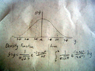
What is the Z statistic? Well consider the graph below:



Suppose we wanted to find the point on the curve that would include 95% of the area. As this happens it is at the point (2 sigma) and the value of the x axis at this point is 1.96 That is to say when x equals 1.96 we capture 95% of the population under the curve. So the Z statistic equals that point on the x-axis or 1.96

Some other common levels of confidence and Z stats are
90% z=1.645
95% z=1.96
98% z=2.33
99% z=2.58

As you see, the Z statistic gets larger and larger as confidence increases. In other words we can be
95% sure that between 77-83% of people prefer wine to cheese
99% sure that between 76-84% of people prefer wine to cheese
and
100% sure that between 0-100% of people prefer wine to cheese (which isn't really saying anything at all)


Now for our example, the mean is 80% and assume the standard error is 1.5% (pretty small really)

to get our confidence interval we take the mean and add the Z stat times the standard error:

u + Z(H) upper limit
u - Z(H) lower limit

80 + 1.96(1.5) upper limit = 80 + 2.94 = 82.94 or rounded to 83%
80 - 1.96(1.5) lower limit = 80 - 2.94 = 77.06 or rounded to 77%

Thus we say with 95% confidence that the mean(u) is

77% < = u < = 83%

Because the mean is 80% we can find the margin of error by subtracting from the top interval.

83%-80% = 3 percent margin of error. Thus we make the statement 80% of people prefer wine to cheese with a 3% margin of error.

The Central Limit Theorem

The central limit theorem states that if a large enough random sample is drawn from a population then the sampling distribution will be normal.

This could be paraphrased as "All sampling distributions become normal distributions when the sample is large enough" and large enough is generally considered to be 20-30 units.



The normal distribution is everywhere in nature.

The Law of Large Numbers

In statistics the law of large numbers states that as sample size increases the accuracy of population estimates increases. This is true for all distributions.

Example:
Suppose we had a bag of 100 marbles and wanted to know how many marbles were solid red.
We could start by drawing 10 marbles from the bag and finding that 2 are red. Thus we estimate that 20% are red.

Then we draw 50 marbles and find that 9 are red, thus we now estimate that 18% are red.

Finally, we draw all 100 marbles (census) and find that there are 17 red marbles. Or that 17% of the marbles are red.

In either case, as we drew more and more marbles our estimate got better and better. This is the law of large numbers.

Sample Means and Deviations

For any random sample (of size n) taken from a population with mean u and standard deviation H

we can say that the mean is equal to X and that the standard deviation is equal to H/sqrt(n)

That is to say, that as the sample (n) gets larger the estimate of the standard deviation will become smaller and more accurate.

Distributions of sample populations are represented by the "t-distribution" that varies in shape by sample size, and looks much like the normal curve covered earlier. As the sample size approaches the population size the t-distribution looks more and more like the normal curve, but that is tomorrow's lesson.