When looking at data
parameters are consider to be measures of the whole population that are fixed, but cannot really be known
statistics are considered to be measures of samples from the population that can be known but can vary and are always inaccurate. The amount of inaccuracy is measured, but even these measures are inaccurate, so probabilities of being correct are often stated, along with possible margins of error
For example, if we stop and randomly ask 100 people their age we might find the average to be 40 years old. This is a statistic because it describes a sample.
However, if we look at the census data for the U.S. we find that the average age is in fact 38. This is a parameter because it theoretically describes the whole population.
Saturday, February 28, 2009
Friday, February 27, 2009
The Normal Distribution (also Gaussian distribution and bell curve)
The Normal distribution is a curve that is symmetric on both sides and centered around the mean of a population. Like all density functions its area under the curve is between 0 and 1.
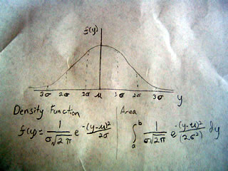
Here the mean is represented by mu, which looks like u and the standard deviation is measured by sigma, which looks like a flat 6.
The chances of being 1 deviation away from the mean are around 30%, 2 deviations is 5%, and 3 deviations is 1%
Like we covered yesterday the probability of values being between any point a and b can be found by taking the area under the curve at those points. The functions are there in the image, and as you can see, they are not fun to evaluate. Thus tables or computers are typically used to help obtain values as opposed to direct calculation.
The curve is also called the Gaussian curve in honor of Carl Friedrich Gauss, the German mathematician who found it. Another name is "Bell curve" since its shape represents a bell.
Thursday, February 26, 2009
Continuous Probability Distributions
So far we have looked at discrete probability distributions where values can be assigned to every outcome in the sample space.
For continuous distributions, probability is represented as a function called the probability density function, or density function. These functions must be greater than zero, and must not have an area greater than 1 under their curves. The functions are called "density functions" because they will graph a smooth curve showing values that are most likely or "dense".
Look at the example below which shows a normal curve:

We can see very quickly that observations are most "dense" between 40 and 50. To find out the exact probability of a value being between 40 and 50, we must calculate the area of the region between 40 and 50. The same is true to find the probability of a value being less than 40. We must calculate the area under the curve that is less than 40. Thus we calculate the area under the curve for any probabilities we want to find.
For continuous distributions, probability is represented as a function called the probability density function, or density function. These functions must be greater than zero, and must not have an area greater than 1 under their curves. The functions are called "density functions" because they will graph a smooth curve showing values that are most likely or "dense".
Look at the example below which shows a normal curve:
We can see very quickly that observations are most "dense" between 40 and 50. To find out the exact probability of a value being between 40 and 50, we must calculate the area of the region between 40 and 50. The same is true to find the probability of a value being less than 40. We must calculate the area under the curve that is less than 40. Thus we calculate the area under the curve for any probabilities we want to find.
Wednesday, February 25, 2009
Geometric Distribution
Suppose we wanted to know the chances of flipping a coin and only seeing a head by the fourth flip, how can we find this?
We can use the geometric distribution which calculates the probability of the number of failures before a success in a Bernouli trail.
The formula is
p(x) = (1-p)xp, where x = 0,1,2,...
Where p(x) is the number of failures, or for our example, the number of tails.
So to apply the formula, what are the chances of flipping a head for the first time on the 4th toss? (This means flipping 3 tails first)
p(x) = number of failures before flipping a head (3)
p(3) = (1 - 0.5)3(0.5) = 0.0625 or around 6%
Pretty low odds!
Monday, February 23, 2009
Binomial Distribution
The binomial distribution is used for multiple Bernouli Trials.
Its formula is written as follows:
p(x) = (n choose x) px * (1-p)n-x , x=0,1,2,....,n
The n choose x part is combinatorial.
n choose x = n! / x!(n-x)! where n is the number of outcomes, and x is the number of outcomes desired.
Example:
Suppose you take a true or false test with 10 questions, what are the chances you get 7 questions right if you just take random guesses? This is a true false so p=50% or .5
p(x) = (10 choose 7) (.5)7*(.5)3
= 10! / 7!*3! *.0078 * 0.125 = 30 * .0078 * 0.125 = 0.029
So you would only have about a 3% chance! Quite amazing. Of course, this means you would have a 97% chance of getting at least 3 wrong, which is not so amazing when you think about it.
Bernoulli Trial
A Bernoulli trial is any experiment in which there can be only two outcomes, usually thought of as a success or failure.
Examples of this can be a coin flip, whether or not you pass a test, or the chances of catching the bus to school.
Assign a 1 to the chance of the event happening, and a 0 to it not happening.
Because discrete distributions have probabilities between 0 and 1, and cannot sum to more than one, a success is defined as p and a failure as 1-p
So the distribution of a Bernoulli trial is seen as
p(x)
0 = 1-p
1 = p
Sunday, February 22, 2009
Discrete Random Variables
It should be known that discrete numbers in mathematics and statistics are not ones that know how to sneak around. Instead, they are countable numbers, even countably infinite numbers. If numbers are not discrete then they are said to be continuous, or uncountable.
In the situation of a coin flip, we can assign a 1 to the outcome of a head, and a 0 to the outcome of a tail. Thus we have transformed the outcome of a coin flip to a discrete random variable, or something that is countable and random.
Discrete distributions must always have probabilities between 0 and 1 and all probabilities must sum to 1.
In math this is
0 < = p(x) < = 1
and Sum(p(x)) = 1
Saturday, February 21, 2009
Bayes Theorem
Bayes theorem is an extension of the theorem of total probability.
Again, we are in a situation where all events in a sample space are mutually exclusive and exhaustive, but this time we want to find conditional probability as opposed to just probability.
We can do this with Bayes theorem which states that the conditional probability of any event (Ei) is
P(Ei,F) = (P(F,Ei)*P(Ei))/(The theorem of total probability)
Recall the theorem of total probability is:
P(F) = P(F and E1) + (F and E2) + (F and E3) + ...(as many as it takes to get "total" probability. "and" in the formula can me taken to mean multiplication or times.)
So in other words we are taking the product of the conditional probability of the outcome, with the probability of the outcome and dividing it by the total probability.
Consider the same example with the factories:
Let us say a company buys parts from 3 other companies.
It gets
60% from company A
40% from company B
20% from company C
Company A ships defective parts 1% of the time (0.01)
Company B ships defective parts 5% of the time (0.05)
Company C ships defective parts 10% of the time (0.10)
Bayes theorem can help us answer the question, what are the chances that a defective part in our company came from company A?
Here the conditional probability of the outcome (defective if from A) is 0.01
The chance of the outcome (bought from A) is 0.60
The probability of any part that is being bought can be found using the total probability theorem. We did that yesterday and found the probability to be 0.046(4.6%)
Bayes theorem says the chances the defective part is from company A is
(0.01*0.60) / 0.046 = 0.13 or 13%
Surprisingly higher than the chance of getting any defective product, but it is because such a large portion of purchases are from that company.
Friday, February 20, 2009
Theorem of Total Probability
Suppose we are in a situation where all events in a sample space are mutually exclusive and exhaustive.
Mutually exclusive means the outcomes are separate from each other, like each time you roll a die.
Exhaustive means all outcomes are accounted for. (You will see in the example)
Example.
Let us say a company buys parts from 3 other companies.
It gets
60% from company A
40% from company B
20% from company C
Company A ships defective parts 1% of the time (0.01)
Company B ships defective parts 5% of the time (0.05)
Company C ships defective parts 10% of the time (0.10)
What are the odds of the company buying a defective part?
Now we have a situation that is exhaustive since all 3 companies comprise 100% of the outcomes. It is also mutually exclusive since one company doesn't affect the other and is "separate".
The theorem of total probability states that when we have an event that is mutually exclusive and exhaustive it can be found by adding the combination of disjoint outcomes. That is to say looking at each company separately and adding them together.
The way to write this is
P(defective part is bought) = P(defective shipped from A) + P(defective shipped from B) + P(defective shipped from C). This represents a "total" account of all outcomes.
The math formula looks like
P(F) = P(F and E1) + (F and E2) + (F and E3) + ...(as many as it takes to get "total" probability. "and" in the formula can me taken to mean multiplication or times.)
The P(defective from a company) is the portion bought from any company times(x) the chance the chance sends something defective.
P(A defective) = 0.6*0.01 = 0.006
P(B defective) = 0.4*0.05 = 0.02
P(C defective) = 0.2*0.10 = 0.02
So
P(defective part is bought) = 0.006 + 0.02 + 0.02 = 0.046 = 4.6%
Thursday, February 19, 2009
Conditional Probability
Conditional probability is used to calculate probability when we have information that can make an event more likely.
For example:
What are the chances of guessing the number rolled on an even 6 sided die?
Since the sample space is {1,2,3,4,5,6} the chances are 1/6
But suppose the person rolling it gave you a hint and told you the number was odd, now what are your chances?
The sample space of odd numbers is {1,3,5} so your chances are 1/3
This is evident in such a small sample space, but we can use a formula for larger sample spaces.
P(E|F) = P(E and F)/P(F)
P(E|F) is read as probability of E given F. In this case E is the chance of guessing the number and F is the chance of the number being odd.
The probability of getting a number that is odd is 1/2 since half the numbers on a six sided die are odd. So P(F)=1/2
The probability of the number being odd and of you guessing the number is still (1/6)
so P(E and F) is 1/6
using the formula, the conditional probability P(E|F) that you can guess the number (E) given that you know it is odd(F) is
P(E|F) = (1/6) / (1/2) = (1/3)
So the formula gives us the same answer we previously saw.
Wednesday, February 18, 2009
P(G or C) = P(G) + P(C) - P(G and C)
P(G or C) = P(G) + P(C) - P(G and C)
When we look for the probability of one event or the other happening we need to add the chance of the first happening with the chance of the second happening, then we need to subtract the probability of both of them happening in order not to over-estimate the chances.
Example:
We are in a store where detailed tracking can tell us the chances of...
a person buying gum P(G) is 0.4
a person buying chocolate P(C) is 0.7
and a person buying both P(G and C) is 0.2
What is the probability that a person buys gum or chocolate?
P(G or C) = P(G) + P(C) - P(G and C)
P(G or C) = 0.4 + 0.7 - 0.2 = 0.9
There is a 90% chance of a customer buying either of those products.
------------------------------
The chances that a customer does not buy gum or chocolate is the complement.
P(not G and not C) = 1 - P(G or C)
or 1 - 0.9 = 0.1 so there is a 10% chance the customer will not buy either...
Tuesday, February 17, 2009
P(E) + P(not E) = 1
P(E) + P(not E) = 1
This is because the probability of any event in the sample space must equal 1. Therefore if we know the probability of E we can also find the probability of not E.
Thus if we want to know the probability of not rolling a 2 on an even die we can say
P(rolling a 2) = 1/6
1/6 + P(not rolling a 2) = 1
P(not rolling a 2) = 1 - (1/6) = (5/6)
Monday, February 16, 2009
Every probability must be greater than or equal to 0 and less than or equal to 1
Every probability must be greater than or equal to 0 and less than or equal to 1
That is to say
0 < = p < = 1
This is because the denominator of any probability is the entire sample space of any outcome.
No outcome, or the null event, would lead to a probability of 0.
That is to say
0 < = p < = 1
This is because the denominator of any probability is the entire sample space of any outcome.
No outcome, or the null event, would lead to a probability of 0.
Sunday, February 15, 2009
Defining and Calculating Probability
Yesterday we looked at sample spaces, outcomes, and events. Today we will look at ways to determine probability.
Again, consider the die. Imagine we wanted to know the probability of rolling an odd number. The sample space for a die is [1,2,3,4,5,6] and the outcomes of rolling an odd number are [1,3,5] so to calculate this probability we take the number of odd outcomes and divide it by the total number of outcomes.
In this case it is 3/6 or 1/2 or 50%. This is only true if the die is not slanted, that is to say, all outcomes are equally likely.
The second way of calculating probability can be used to test if the die is honest. This is found by rolling the die many times, around 100 and seeing how many times an odd number comes up. So in this case we calculate the probability by counting the number of times an odd number occurs over the number of times we roll the die.
Suppose we do this 100 times and find we rolled 55 odd numbers. Then we see that 55/100 times we rolled an odd, or 55% of the time. This is close enough to 50% to say that the die is honest. After rolling the die 1000 times or even 10,000 times we would expect the number to get closer and closer to 50%.
This second method of probability can also be used in times we we do not know the sample space. Let us say we want to know the probability of making a sale when a customer walks into our shop. There is no way to calculate this theoretically(the first method) and we must do it by counting. Assume that 100 people walk into the shop, and only 20 people end up making a purchase, then we conclude that the probability of making a sale is 20/100 or 20%.
Saturday, February 14, 2009
Probability: Events, Outcomes, and Sample Spaces
Probability is one of the least intuitive aspects of statistics. If it wasn't, Casinos wouldn't net the billions of dollars they do each year.
What do we need to know to get a grounding in probability?
The first thing is the sample space, this is the set of all possible outcomes. For a coin it is heads or tails, for a die it is [1,2,3,4,5,6] and for the height of a person it is [x:x>0]
Outcomes are the result of any random event that we want to predict, i.e. we roll a die and a 2 comes up.
An Event is a desired outcome and is often denoted with a capital letter. For the dice we can define the event, A, as A=2.
Imagine we roll the die again and a 5 is the outcome. Then our desired event did not happen.
Bivariate Data
Bivariate data is a fancy way of saying "data with two variables".
Variables can be anything:
number of apples and number of oranges
number of church goers and number of bibles
number of ciggies smoked and number of people with cancer
number of guns and amount of ammo
number of plastic toys sold and number of cartoons
From this list we can see that bivariate data is suggestive. Did you hear yourself say: "Yeah, totally related, that definitely causes the other".
And so comes one of the most notorious dilemmas in statistics: Causation vs. Correlation.
Causation means that one causes the other, like the more you drive your car, the less gas you have in the tank.
Correlation is mere chance, but not related. For example, if we were to look at the number of people paying taxes and the number of people who die we would find a pretty good correlation, but, this doesn't count since taxes don't kill you...no matter how convinced you are that they do.
Consider this example:
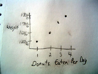
Here we see that the more donuts a person eats per day, the higher their weight. Does that really mean that eating more donuts will mean you weigh more? What about other factors like exercise? To get a better appreciation of what is happening, it might be best to include exercise and create a multivariate model, but we will cover that later.
Variables can be anything:
number of apples and number of oranges
number of church goers and number of bibles
number of ciggies smoked and number of people with cancer
number of guns and amount of ammo
number of plastic toys sold and number of cartoons
From this list we can see that bivariate data is suggestive. Did you hear yourself say: "Yeah, totally related, that definitely causes the other".
And so comes one of the most notorious dilemmas in statistics: Causation vs. Correlation.
Causation means that one causes the other, like the more you drive your car, the less gas you have in the tank.
Correlation is mere chance, but not related. For example, if we were to look at the number of people paying taxes and the number of people who die we would find a pretty good correlation, but, this doesn't count since taxes don't kill you...no matter how convinced you are that they do.
Consider this example:
Here we see that the more donuts a person eats per day, the higher their weight. Does that really mean that eating more donuts will mean you weigh more? What about other factors like exercise? To get a better appreciation of what is happening, it might be best to include exercise and create a multivariate model, but we will cover that later.
Thursday, February 12, 2009
Measuring dispersion in Sample Data
Various tools can be used in measuring dispersion in sample data, because it is unlikely that any sample will contain the absolute lowest and highest value on the population it can tend to underestimate actual dispersion.
The formula to calculate sample variance is similar to variance and is written as:
s2 = 1/(n-1) * sum(X(values)-mean))2
The only difference is that we divide by n-1 instead of n, because sample variance tends to be an underestimate.
Other tools to measure sample variance are quartiles or percentiles.
The median can be thought as the 50th percentile, since 50 of the values fall both above and below it. Thus with the 75th percentile, 75% of the values fall below it and 25% are above it, and so on. These simple percentiles can give a good estimate of dispersion in the sample.
Wednesday, February 11, 2009
Variance and Standard Error
In addition to dispersion we can also measure distribution of data with variance and standard error.
The variance is found by subtracting each observation from the mean, squaring it, then summing them all together. Mathematically this is:
Variance = Sum(n-u)^2/N
were n is any observation, and u is the mean.
The Standard deviation is simply the square root of this number.
The variance is found by subtracting each observation from the mean, squaring it, then summing them all together. Mathematically this is:
Variance = Sum(n-u)^2/N
were n is any observation, and u is the mean.
The Standard deviation is simply the square root of this number.
Tuesday, February 10, 2009
Measuring dispersion
Yesterday we talked about measuring central tendency. This is a good statistic, but it is even better when it is partnered with its side kick: dispersion.
Consider the diagram:
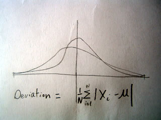
As we can see, the two distributions of data have similar central tendencies, but different amounts of dispersion.
One way to measure dispersion is to take the average of each value in the data set subtracted from the mean, using the formula shown in the picture.
Notice the symbol for summation of the absolute value of all observations subtracted from the mean.
Consider the diagram:
As we can see, the two distributions of data have similar central tendencies, but different amounts of dispersion.
One way to measure dispersion is to take the average of each value in the data set subtracted from the mean, using the formula shown in the picture.
Notice the symbol for summation of the absolute value of all observations subtracted from the mean.
Monday, February 9, 2009
Measures of Central Tendency in Numerical Data
Measuring central tendency in a distribution of data(numbers) provides a one-digit statistic, or descriptive source of information, that convey a lot of information about that data.
It is not as complicated as it sounds, consider the three most common ways of measuring central tendency: mean(average),median, and mode.
Consider a set of numerical data {1,3,4,5,5,6,6,7,8,10) N=10
Capital N is commonly used to represent the total number in the set(population) of data(the sample).
The mean, or average, is found by adding all elements of the data and then dividing by the total number in the set.
Thus
mean = 1+3+4+5+5+6+6+7+8+10/10 = 55/10 = 5.5
So the mean or average is 5.5
The median is found by ordering the numbers from lowest to highest and locating the value in the middle.
In this case, both 5 and 6 are in the middle, thus the median is the average of the two or 5+6/2 = 5.5
The mode is the most frequent value in the data set. For our example set it both 5 and 6 appear twice, and thus, they are both the mode.
It is no accident that the mean, median, and mode produce numbers which are either equal or close. Measures of central tendency are similar, after all the number which appears most (mode) is expected to most affect the average.
Sunday, February 8, 2009
Frequency and Relative frequency, (Counts and percentages)
Frequencies are probably the most popular statistics.
A frequency is nothing more than a count.
And a relative frequency is a percentage.
Thus if we have a sample of 10 marbles we may count
4 red marbles
3 green marbles
2 blue marbles
1 yellow marble
The 4,3,2,1 are their counts or frequencies and their relative frequency would be the percentage they represent of the sample of 10.
We find a percentage dividing the count by the sample size, like
4/10 = 0.4 or 40%
4/10 = 0.2 or 30%
4/10 = 0.3 or 20%
4/10 = 0.1 or 10%
Data like this is often seen in the form of a bar chart, or a pie chart and is one of the most popular ways to present data for drawing conclusions.
Saturday, February 7, 2009
Statistics, Basic Concept and Key Terms
The next series of days will focus on Statistics.
Statistics is the science and art of collecting, analyzing, and making conclusions about data. All data is collected from a set population. Subsets of the population can be called members, or units. If every subset of the population is collected, then we have a census, however, often just a small portion of the population is sampled. The sample is then thought to represent the whole population.
Care must be taken when choosing any given sample. For example, if we want to get an idea of how a population will vote on a new cigarette tax it does no good to sample non-voters like children. Also, the sample must be random in order to assure accurate results. If we only ask voters leaving a cigarette store, we are not likely to get good results and arrive to correct conclusions.
Friday, February 6, 2009
Proof of Herons Formula to find the area of a non-right triangle
Proof of Herons Formula to find the area of a non-right triangle
Consider the following triangle:
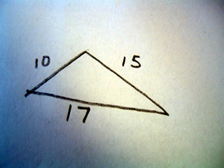
There are no right angles in the triangle, so therefore we must use Heron's forumla which first defines a variable s
s=1/2(a+b+c) where a,b,c each represent the length of a side.
then the area of the triangle is equal to
sqrt(s(s-a)(s-b)(s-c))
For the example we see that s=21
and the area is equal to
sqrt(21(21-10)(21-15)(21-17))
=
sqrt(21*11*6*4)=sqrt(5,544)=~74.46 which is the area of the triangle.
How do we prove Herons formula? Consider the triangle:
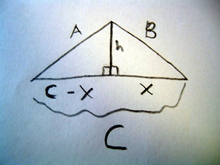
Here we have taken a triangle with no right angles, and cut a line so that we create two right triangles, and two new lengths at the base: x, and C-x. Now we need to solve for two unknown values x and h. We will solve for x first.
We can use pythagorean theorem to create equations for our new values, we see we have:
x2 + h2 = B2
and
(c-x)2 + h2 = A2
=
C2 - 2cx + x2+ h2 = A2
We know that B= x2+h2 so we substitute that in to the equation above and get
C2 - 2cx + B2 = A2
Now we can solve for x!
x= (A2 - B2 - C2) / - 2c
Now we have x we can plug it back in to the equation
x2 + h2 = B2
thus
h = sqrt(B2 - (A2 - B2 - C2) / - 2c)2)
Now, we know our base is equal to C and our height is equal to h, if we substitute these two values into the formula for the area of a triangle we get
(1/2)*b*h = 1/2*C2*sqrt(B2 - (A2 - B2 - C2) / - 2c)2)
That is a complicated formula, so Heron found that you could define a term
s = (1/2)*( A + B + C) and then found the area formula could become a simpler
sqrt(s(s-a)(s-b)(s-c))
If you plug s in to the area formula above you will find the result we saw above:
1/2*C2*sqrt(B2 - (A2 - B2 - C2) / - 2c)2)
which is the area of the triangle.
Consider the following triangle:
There are no right angles in the triangle, so therefore we must use Heron's forumla which first defines a variable s
s=1/2(a+b+c) where a,b,c each represent the length of a side.
then the area of the triangle is equal to
sqrt(s(s-a)(s-b)(s-c))
For the example we see that s=21
and the area is equal to
sqrt(21(21-10)(21-15)(21-17))
=
sqrt(21*11*6*4)=sqrt(5,544)=~74.46 which is the area of the triangle.
How do we prove Herons formula? Consider the triangle:
Here we have taken a triangle with no right angles, and cut a line so that we create two right triangles, and two new lengths at the base: x, and C-x. Now we need to solve for two unknown values x and h. We will solve for x first.
We can use pythagorean theorem to create equations for our new values, we see we have:
x2 + h2 = B2
and
(c-x)2 + h2 = A2
=
C2 - 2cx + x2+ h2 = A2
We know that B= x2+h2 so we substitute that in to the equation above and get
C2 - 2cx + B2 = A2
Now we can solve for x!
x= (A2 - B2 - C2) / - 2c
Now we have x we can plug it back in to the equation
x2 + h2 = B2
thus
h = sqrt(B2 - (A2 - B2 - C2) / - 2c)2)
Now, we know our base is equal to C and our height is equal to h, if we substitute these two values into the formula for the area of a triangle we get
(1/2)*b*h = 1/2*C2*sqrt(B2 - (A2 - B2 - C2) / - 2c)2)
That is a complicated formula, so Heron found that you could define a term
s = (1/2)*( A + B + C) and then found the area formula could become a simpler
sqrt(s(s-a)(s-b)(s-c))
If you plug s in to the area formula above you will find the result we saw above:
1/2*C2*sqrt(B2 - (A2 - B2 - C2) / - 2c)2)
which is the area of the triangle.
Thursday, February 5, 2009
Prove the area of a right triangle is equal to half the base*height
Prove that the area of a triangle is equal to 1/2*base*height.
The essence of this proof is to show that any right triangle can be made into a rectangle of the same base and height.
Consider the following two triangles:
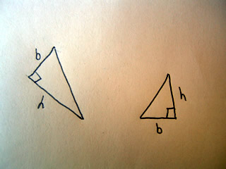
Both these triangles can be made into rectangles with the same base and height as shown below:
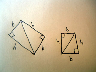
The area of a rectangle is length times width, or in this case base times height.
The hypotenuse of the triangle cuts the rectangle directly in half, and thus the area of a triangle is 1/2 of a rectangle, or 1/2 base times height.
The essence of this proof is to show that any right triangle can be made into a rectangle of the same base and height.
Consider the following two triangles:
Both these triangles can be made into rectangles with the same base and height as shown below:
The area of a rectangle is length times width, or in this case base times height.
The hypotenuse of the triangle cuts the rectangle directly in half, and thus the area of a triangle is 1/2 of a rectangle, or 1/2 base times height.
Wednesday, February 4, 2009
The Law of Cosines
When we know the length of two sides of a triangle, and the angle between them, we can use the law of cosines to find the length of the remaining side.
The law of cosines states:
C^2 = A^2 + B^2 - 2AB*cos(theta)
Here is an example of the law of cosines:

Proof of the Law of Cosines
The law of cosines looks similar to the pythagorean theorem (C^2 = A^2 + B^2) and indeed the two are similar. What we have to do to prove the law of cosines is to create a right triangle and define coordinates for that right triangle so we can find our remaining side.
Consider the diagram below:

Imagine the triangle on a coordinate plane. We define the origin, the point (0,0) at the end of side B. Thus the coordinate to the left is (-B,0). The coordinate at the top of the triangle (A*cos(theta)-B,A*sin(theta)) is derived from the right triangle sketch in on the right of our triangle. Although the coordinates appear complex, keep in mind they represent two numbers:
(A*cos(theta)-B,A*sin(theta)) is equal to some (x,y) on the coordinate plane.
Now that we have defined some coordinates we can draw a line down from the top angle to some point on side B, this creates a right triangle as shown below.
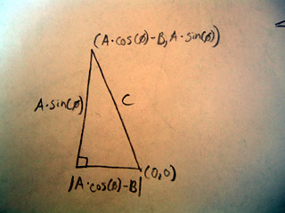
Using the coordinates which we defined we can define the length of the sides of this triangle.
The bottom side has length: |A*cos(theta)-B|.
A*cos(theta) comes from the dotted triangle we sketched in the previous image and represents the length that we have chopped off of side B. This the new length of the triangle is A*cos(theta)-B , it could also be B-A*cos(theta). Because we don't know which way to subtract, we take the absolute value so that both equations give us the same length, and write the distance as |A*cos(theta)-B|. The length of the vertical side also comes from the previous dotted triangle, and is simply A*sin(theta).
With these lengths now defined we can find C with the pythagorean theorem.
C2= (A*sin(theta)2 + (A*cos(theta) - B)2
Mutliply this out and you get
C2=A2*sin2(theta) +A2cos2(theta) - 2AB*cos(theta) + B2
Factoring out the A2 we get
C2=A2(sin2(theta)+cos2(theta))-2AB*cos(theta)+B2
Knowing that sin2(theta)+cos2(theta)=1 we get
C2=A2 - 2AB*cos(theta) + B2
whic is the Law of Cosines.
C2 = A2 + B2 - 2AB*cos(theta)
The law of cosines states:
C^2 = A^2 + B^2 - 2AB*cos(theta)
Here is an example of the law of cosines:
Proof of the Law of Cosines
The law of cosines looks similar to the pythagorean theorem (C^2 = A^2 + B^2) and indeed the two are similar. What we have to do to prove the law of cosines is to create a right triangle and define coordinates for that right triangle so we can find our remaining side.
Consider the diagram below:
Imagine the triangle on a coordinate plane. We define the origin, the point (0,0) at the end of side B. Thus the coordinate to the left is (-B,0). The coordinate at the top of the triangle (A*cos(theta)-B,A*sin(theta)) is derived from the right triangle sketch in on the right of our triangle. Although the coordinates appear complex, keep in mind they represent two numbers:
(A*cos(theta)-B,A*sin(theta)) is equal to some (x,y) on the coordinate plane.
Now that we have defined some coordinates we can draw a line down from the top angle to some point on side B, this creates a right triangle as shown below.
Using the coordinates which we defined we can define the length of the sides of this triangle.
The bottom side has length: |A*cos(theta)-B|.
A*cos(theta) comes from the dotted triangle we sketched in the previous image and represents the length that we have chopped off of side B. This the new length of the triangle is A*cos(theta)-B , it could also be B-A*cos(theta). Because we don't know which way to subtract, we take the absolute value so that both equations give us the same length, and write the distance as |A*cos(theta)-B|. The length of the vertical side also comes from the previous dotted triangle, and is simply A*sin(theta).
With these lengths now defined we can find C with the pythagorean theorem.
C2= (A*sin(theta)2 + (A*cos(theta) - B)2
Mutliply this out and you get
C2=A2*sin2(theta) +A2cos2(theta) - 2AB*cos(theta) + B2
Factoring out the A2 we get
C2=A2(sin2(theta)+cos2(theta))-2AB*cos(theta)+B2
Knowing that sin2(theta)+cos2(theta)=1 we get
C2=A2 - 2AB*cos(theta) + B2
whic is the Law of Cosines.
C2 = A2 + B2 - 2AB*cos(theta)
Tuesday, February 3, 2009
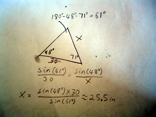
The Law of Sines
When we know the measure of the angles of a triangle, and the measure of one of its sides, we can use the law of sines to find the length of the other two sides.
The law sines states for any triangle with sides A,B, or C that
sin(a)/A = sin(b)/B = sin(c)/C
or equivalently
A/sin(a) = B/sin(b) = C/sin(c)
So if we have a triangle as such, with side x unknown we can find it by using the law of sines:
Proof of the Law of Sines
Consider the following diagram:
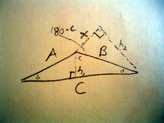
In the first step of the proof we divide the triangle into two right triangles by drawing a line of length h1.
Now we have two right triangles we can say that
sin(b)=h/A or h=A*sin(b)
similarly
sin(a)=h/B so h=B*sin(a)
now we can see that
B*sin(a)=h=A*sin(b)
divide both sides by AB and we get
sin(a)/A = sin(b)/B which is the first half of the law of sines.
For the next part, we draw a right triangle out from side B, creating a new length h2.
From this new triangle we see that
sin(b)=h/C and h=sin(b)*C
we also see that
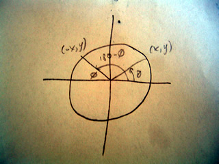
sin(180-c) = h/B or h=sin(180-c)*B
but from the unit circle below we see that sin(180-c)=sin(c)
so we can write sin(c)*B=h and from this conclude
sin(b)*C=h=sin(c)*B
again we divide both sides by BC and get
sin(b)/B = sin(c)/C
so we have sin(a)/A=sin(b)/B=sin(c)/C which is the law of sines.
The law sines states for any triangle with sides A,B, or C that
sin(a)/A = sin(b)/B = sin(c)/C
or equivalently
A/sin(a) = B/sin(b) = C/sin(c)
So if we have a triangle as such, with side x unknown we can find it by using the law of sines:
Proof of the Law of Sines
Consider the following diagram:
In the first step of the proof we divide the triangle into two right triangles by drawing a line of length h1.
Now we have two right triangles we can say that
sin(b)=h/A or h=A*sin(b)
similarly
sin(a)=h/B so h=B*sin(a)
now we can see that
B*sin(a)=h=A*sin(b)
divide both sides by AB and we get
sin(a)/A = sin(b)/B which is the first half of the law of sines.
For the next part, we draw a right triangle out from side B, creating a new length h2.
From this new triangle we see that
sin(b)=h/C and h=sin(b)*C
we also see that
sin(180-c) = h/B or h=sin(180-c)*B
but from the unit circle below we see that sin(180-c)=sin(c)
so we can write sin(c)*B=h and from this conclude
sin(b)*C=h=sin(c)*B
again we divide both sides by BC and get
sin(b)/B = sin(c)/C
so we have sin(a)/A=sin(b)/B=sin(c)/C which is the law of sines.
Monday, February 2, 2009
An Example of Vector Physics
Assume you try to pull a box across the room. You exert 150 pounds of pressure (which you could measure with a spring) on the box, how much force will be used to drag the box and how much to lift it? This problem can be solved with trigonometry.

Thus from the sketch we see we can calculate horizontal force as
150 * cos(40) = 115 lbs of force
We get this equation knowing that the cosine of an angle is adjacent over hypotenuse, thus
adjacent = hypotenuse*cosine(angle)
or
115 = 150 * cos(40)
By the same method we can find the opposite side which will give us the force of lift.
150 * sin(40) = 96 pounds
Whether or not this is enough force to move the box depends on the friction and weight of the box, as well as several other variables.
Sunday, February 1, 2009
Vectors
Vectors in math are lines which represent both distance, and direction. They can also be used to represent magnitude or force.
A Vector:

A Vector:
Subscribe to:
Posts (Atom)